Types of B-Tree Indexes are:
- Descending index
- Key Composite Index
- Reverse Key Index
- B-Tree cluster Index
- Index Organized Table(IOT)
Descending Index
In B* Tree indexes by default, data is stored in ascending order, character data is ordered by binary values contained in each byte of the value, numeric data from smallest to largest number, and date from earliest to latest value.
You can create a descending index by specifying the DESC keyword in the CREATE INDEX statement. In this case, the index stores the index data in descending order. In this case the Rightmost index leaf will have the lowest value and left most leaf node will have maximum value.
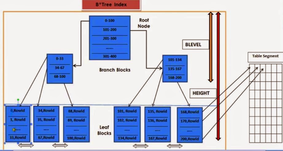
As can be seen from Diagram, by default data is stored in Ascending order. In Left most block value is 0,1,..33 and in the rightmost we have bigger values 168, 170, 200.
In case of DESCENDING it will be reversal. In Left most it will have greater values and in rightmost block it will have lower values.
Proc & Cons:
Descending indexes are useful when you are using composite index on some columns and the query sorts some columns ascending and some query descending.
First we will create a table and then a normal ascending Index on it.
SQL> CREATE TABLE T_OBJ AS SELECT * FROM ALL_OBJECTS;
Table created.
SQL> CREATE INDEX T_OBJ_INDX ON T_OBJ(OBJECT_TYPE, OBJECT_ID, OBJECT_NAME);
Index created.
Gather statistics:
SQL> BEGIN
SYS.DBMS_STATS.GATHER_TABLE_STATS(
OwnName => 'SCOTT',
TabName => 'T_OBJ',
Estimate_Percent => 0,
Method_opt => 'for all indexed columns',
Cascade => TRUE,
No_Invalidate => FALSE);
END;
/
PL/SQL procedure successfully completed.
SELECT OBJECT_TYPE, OBJECT_ID, OBJECT_NAME
FROM T_OBJ
WHERE OBJECT_TYPE = 'TABLE'
AND OBJECT_ID < 1000
ORDER BY OBJECT_TYPE DESC, OBJECT_ID DESC, OBJECT_NAME DESC;

It is doing Index Range Scan Desceding and then it is giving us the data. This means oracle has the ability to scan the index in descending order.By default it is ascending.
Now executing query again but making OBJECT_ID order Ascending.
SELECT OBJECT_TYPE, OBJECT_ID, OBJECT_NAME
FROM T_OBJ
WHERE OBJECT_TYPE = 'TABLE'
AND OBJECT_ID < 1000
ORDER BY OBJECT_TYPE DESC, OBJECT_ID ASC, OBJECT_NAME DESC;

It is doing INDEX RANGE SCAN and then SORT ORDER BY to give you the sorted data because two column I am ordering by descending and one column in ascending order.
Now creating a Descending Index:
DROP INDEX T_OBJ_INDX;
CREATE INDEX T_OBJ_INDX ON T_OBJ(OBJECT_TYPE DESC, OBJECT_ID ASC, OBJECT_NAME DESC);

Now this time it is doing only INDEX RANGE SCAN and it has eliminated the step SORT ORDER BY. So this is the benifit of Descending index.
Key Compressed Index
Another interesting feature of B*Tree index is index key compression. Creating an index using key compression enables you to eliminate duplicate occurences of index key values in a B*Tree indexes or IOT. Key compression is useful when the database deals with duplicates in the index keys.
The basic idea behind a key compression is that every entry is broken into two pieces: a prefix and a suffix component. The prefix is built on the leading columns of the composite index and will have repeating values. The suffix is built on the trailing columns in the index key and is the unique or almost unique component of the index entry. The database achieves compression by sharing the prefix entries among the suffix entries in an index block.
CREATE INDEX T_OBJ_INDX_NONCOMPRESS
ON T_OBJ(OWNER, OBJECT_TYPE, OBJECT_NAME);
Conceptually a noncompressed index leaf block stores index key, rowid combination like this diagram. Leaf block entry will look like this:

Owner, Object_Type, Object_Name and Rowid
Analyzing index to populate index stats:
ANALYZE INDEX T_OBJ_INDX_NONCOMPRESS VALIDATE STRUCTURE;
CREATE TABLE T_INDX_STATS
AS SELECT NAME, HEIGHT, LF_BLKS, BR_BLKS, BTREE_SPACE, OPT_CMPR_COUNT, OPT_CMPR_PCTSAVE
FROM INDEX_STATS;
Index stats will be updated once we update the structure and old value will be removed. So we are storing stats in TABLE T_INDX_STATS.
SELECT * FROM T_INDX_STATS;
NAME HEIGHT LF_BLKS BR_BLKS BTREE_SPACE OPT_CMPR_COUNT OPT_CMPR_PCTSAVE
------------------------------ ---------- ---------- ---------- ----------- -------------- ----------------
T_OBJ_INDX_NONCOMPRESS 3 403 3 3248096 2 28
OPT_CMPR_COUNT and OPT_CMPR_PCTSAVE are related with compression. BTREE_SPACE is total space of the index.
Now dropping this non-compressed index and creating a new index with compression of 1.
DROP INDEX T_OBJ_INDX_NONCOMPRESS;
CREATE INDEX T_OBJ_INDX_COMPRESS_1 ON T_OBJ(OWNER, OBJECT_TYPE, OBJECT_NAME) COMPRESS 1;
ANALYZE INDEX T_OBJ_INDX_COMPRESS_1 VALIDATE STRUCTURE;
INSERT INTO T_INDX_STATS
SELECT NAME, HEIGHT, LF_BLKS, BR_BLKS, BTREE_SPACE, OPT_CMPR_COUNT, OPT_CMPR_PCTSAVE
FROM INDEX_STATS;
Populating the index stats again:
SELECT * FROM T_INDX_STATS;
SQL> SELECT * FROM T_INDX_STATS;
NAME HEIGHT LF_BLKS BR_BLKS BTREE_SPACE OPT_CMPR_COUNT OPT_CMPR_PCTSAVE
------------------------------ ---------- ---------- ---------- ----------- -------------- ----------------
T_OBJ_INDX_NONCOMPRESS 3 403 3 3248096 2 28
T_OBJ_INDX_COMPRESS_1 3 359 3 2894660 2 19
As we can see number of Leaf Block have reduced. And the amount of Btree space is also reduced.
OPT_CMPR_COUNT = optimum compression percent saved.
OPT_CMPR_PCTSAVE = Estimated compression count which is best suitable for key compression on the index. 28 shows we can save 28% of space with this index. Second method shows, we have saved some space with this index and we can save 19% more.

Diagram shows, if we use specify prefix length = 1 by using Compress 1 then it will look like this. Prefix entry will be there once on the leaf block not once per repeated entry. If we use compression, each suffix entry references a prefix entry, which is stored in the same index block as the suffix entry.
Here prefix will be Sys. Leaf block will have entry as PROCEDURE, OBJE_NAME, ROWID.
Now creating Index with compression count of 2:
DROP INDEX T_OBJ_INDX_COMPRESS_1;
CREATE INDEX T_OBJ_INDX_COMPRESS_2 ON T_OBJ(OWNER, OBJECT_TYPE, OBJECT_NAME) COMPRESS 2;
ANALYZE INDEX T_OBJ_INDX_COMPRESS_2 VALIDATE STRUCTURE;
INSERT INTO T_INDX_STATS
SELECT NAME, HEIGHT, LF_BLKS, BR_BLKS, BTREE_SPACE, OPT_CMPR_COUNT, OPT_CMPR_PCTSAVE
FROM INDEX_STATS;
Checking the stats with compression 2:
SQL> SELECT * FROM T_INDX_STATS;
NAME HEIGHT LF_BLKS BR_BLKS BTREE_SPACE OPT_CMPR_COUNT OPT_CMPR_PCTSAVE
------------------------------ ---------- ---------- ---------- ----------- -------------- ----------------
T_OBJ_INDX_NONCOMPRESS 3 403 3 3248096 2 28
T_OBJ_INDX_COMPRESS_1 3 359 3 2894660 2 19
T_OBJ_INDX_COMPRESS_2 3 288 3 2326944 2 0
Leaf block have reduced much more. And OPT_CMPR_PCTSAVE is showing 0 that mean you cannot save anymore space if you use a larger compression degree. You have all the space you could save in compression.

If we use compression 2 then conceptually it will look like this. Prefix entry will contain the owner, object_type combination and Suffix entry will be object_name. Each suffix entry points to the prefix entry(owner, object_type).
Now creating Index with compression count of 3:
DROP INDEX T_OBJ_INDX_COMPRESS_2;
CREATE INDEX T_OBJ_INDX_COMPRESS_3 ON T_OBJ(OWNER, OBJECT_TYPE, OBJECT_NAME) COMPRESS 3;
ANALYZE INDEX T_OBJ_INDX_COMPRESS_3 VALIDATE STRUCTURE;
INSERT INTO T_INDX_STATS
SELECT NAME, HEIGHT, LF_BLKS, BR_BLKS, BTREE_SPACE, OPT_CMPR_COUNT, OPT_CMPR_PCTSAVE
FROM INDEX_STATS;
Checking the stats with compression 2:
SQL> SELECT * FROM T_INDX_STATS;
NAME HEIGHT LF_BLKS BR_BLKS BTREE_SPACE OPT_CMPR_COUNT OPT_CMPR_PCTSAVE
------------------------------ ---------- ---------- ---------- ----------- -------------- ----------------
T_OBJ_INDX_NONCOMPRESS 3 403 3 3248096 2 28
T_OBJ_INDX_COMPRESS_1 3 359 3 2894660 2 19
T_OBJ_INDX_COMPRESS_2 3 288 3 2326944 2 0
T_OBJ_INDX_COMPRESS_3 3 450 3 3622296 2 35
As you can see, the number of Leaf Block have actually increased than the first one with non-compressed index. The BTree space have also incrased. OPT_CMPR_PCTSAVE is 35. So it is not the obtimal compression that you can do. Compress 2 was the best one. BTREE_SPACE with compression 2 was 2326944, but with compression =3 it will be 35% increase in BTREE_SPACE in compression 2.

If we use compress 3 then conceptually it will look like this. Prefix entry will contain the owner, object_type, object_name combination. By using compression 3 it will add the object_name in the prefix entry itself, which will make it almost unique.
Therefore its like adding a additional prefix entry to almost all index Key & makes it almost uniqe, because of this the number of leaf blocks & size of index will grow.
Default Compression
Creating a Index without specifying any Compress.
DROP INDEX T_OBJ_INDX_COMPRESS_3;
CREATE INDEX T_OBJ_INDX_COMPRESS_DF ON T_OBJ(OWNER, OBJECT_TYPE, OBJECT_NAME) COMPRESS 3;
ANALYZE INDEX T_OBJ_INDX_COMPRESS_DF VALIDATE STRUCTURE;
INSERT INTO T_INDX_STATS
SELECT NAME, HEIGHT, LF_BLKS, BR_BLKS, BTREE_SPACE, OPT_CMPR_COUNT, OPT_CMPR_PCTSAVE
FROM INDEX_STATS;
SQL> SELECT * FROM T_INDX_STATS;
NAME HEIGHT LF_BLKS BR_BLKS BTREE_SPACE OPT_CMPR_COUNT OPT_CMPR_PCTSAVE
------------------------------ ---------- ---------- ---------- ----------- -------------- ----------------
T_OBJ_INDX_NONCOMPRESS 3 403 3 3248096 2 28
T_OBJ_INDX_COMPRESS_1 3 359 3 2894660 2 19
T_OBJ_INDX_COMPRESS_2 3 288 3 2326944 2 0
T_OBJ_INDX_COMPRESS_3 3 450 3 3622296 2 35
T_OBJ_INDX_COMPRESS_DF 3 450 3 3622296 2 35
Here we can observe that there is no difference between compress index 3 and the default compression. But it is not the optimal compression. The optimal compression is with Compress = 2.
Key Compress Index Proc & Cons:
- Can Reduce Index storage spac.
- In Key compressed index there will be more index entries per leaf block, it can reduce Logical IO, lache and increase buffer cache efficiently as same time ths reason also can cause block contention on frequency modified tables and it may take little more CPU process to use the index in some cases.
Reverse Key Indexes
A reverse key Index is a type of B-Tree index that physically reverse the bytes of each index key.
They were implemented to reduce block contention on index leaf blocks in indexes, specifically on column populated by a sequence, specially in a Oracle RAC Environment.
Indexes are sorted (Key, ROWID) pair, meaning values in the index are arranged in ascending or descending key order. ROWID in the leaf block points to specific rows in the table segment with that index values. In the case of Unique/PK columns, when populated by sequence based key values, recent entries will be in the rightmost leaf block of the B-Tree. All new data will be sorted in the right most block of the index. As using the sequence more and more sessions insert rows into the table, that right most leaf block will be full, then oracle will split the right most lead block into two leaf blocks: One row with all rows except one row and new block with just one row. Now that new leaf block becomes the right most leaf block and the concurrency moves to the new leaf block. This type of index growth is termed as "Right Hand Growth" indexes.
As sessions inserts in to the right most leaf block of index, it becomes the hot block, and cause contention on that leaf block which lead to Buffer Busy Wait. In RAC environment the problem can become dangerous. While inserting values from sequence, that hot - right most index leaf block will be transferred between the instances. If the block is considered busy, then LMS process might induce more delay in transferring the blocks between the instances. While the block is in transit, then the session accessing that block will face GC buffer busy waits and excessive GC Buffer Busy can very much significant performance issue.
"Reverse Key Indexes" are designed to resolve this issue related to index block contention. It physically reverses the byte of each index key. While DML operation Reverse Key Index simply takes the index column values and reverse the key value & insert in the Leaf Node. Reversing the key of the index allows insertions to be distributed across all the leaf blocks in the index which can make insertion faster because there will be no block contension.
How Reversing Works:
Suppose the right most leaf block in the B-Tree has values as 368, 369, 370 and so on. These values are populates using Sequence.
Now the internal representation of 368 will be [c2,4,45], for 369 it will be [c2,4,46], for 370 it will be [c2,4,47]. We can see that first two values [c2,4] is almost same in all these values and only the last value (45, 46, 47) changes.
In case of Reverse Key Indexes, oracle will reverse these values. [c2,4,45] will become [45,4,c2] and [c2,4,46] will become [46,4,c2]. So these values are not adjusent anymore. This is the way oracle will distribute. When insertion [c2,4,46] will come and it will become [46,4,c2] and oracle might put it in different block according to particular order. Similarly, for another value 371 value is [c2,4,48], then Oracle will reverse it as 48,4,c2 and then oracle will place it in some other block not in the right most leaf block.
So based on the Reverse value the order will be maintained, but based on the actual key value there will be no order. As the new value are inserted, the insertion will be distributed across all different leaf nodes, then there will be no block contention on the leaf block. This way we can eliminate Block Contension.
To create a reverse key index, use the REVERSE clause.
CREATE INDEX empno_idx ON emp(empno) REVERSE;
It is possible to make an existing index a reverse key index with the ALTER INDEX command.
ALTER INDEX emp_pk REBUILD REVERSE;
To make the index a normal index again, use the NOREVERSE clause.
ALTER INDEX emp_pk REBUILD NOREVERSE;
Reverse Key Index - Proc and Cons
While DML operation Reverse Key Index simply takes the index column values and reverse the key value & insert in the Leaf node. Reversing the key of the index allows insertions to be distributed across all the leaf blocks in the index which can make insertion faster.
As the index is not sorted by column key, One problem with Reverse key Index is processing Range Predicates in your query (e.g. BETWEEN, >, <, >=, <=, LIKE etc.). While using Reverse key index CBO totally ignores Reverse Key Indexes when processing Range Predicates.
B Tree Clustered Index
Clustering is a feature in Oracle using which you can store a group of tables that share common column, in the same database blocks and store related data together on the same block. With a cluster a simple data block may contain data from many tables. You can create a Cluster key on the common column.
Clustering is very much useful when you have some tables with common columns, and frequently you use that column to join the tables to fetch data.
The Cluster Index is a B-Tree index on the cluster key. A cluster index must be created before any rows can be inserted into clustered tables.
For example you have Employees and Department Table. You use Department_Id to join these two tables. You join these tables and fetch data very frequently. For this scenario we can consider creating a cluster and you will create a Cluster Key on the Department_Id. You create a Clustered Index (B*Tree cluster) on this Department_Id, and you create two cluster table Employee and Department in the cluster.
Create a Cluster:
CREATE CLUSTER emp_dept_cluster
(DeptNo NUMBER(4))
SIZE 512;
Create B Tree Clustered Index:
CREATE INDEX Emp_Dept_Cluster_Indx ON CLUSTER emp_dept_cluster;
Now create two Clustered Table on this cluster:
create table emp_c(
empno number(4,0) PRIMARY KEY,
ename varchar2(10),
job varchar2(9),
mgr number(4,0),
hiredate date,
sal number(7,2),
comm number(7,2),
deptno number(4,0))
CLUSTER emp_dept_cluster(DeptNo);
create table dept_c(
deptno number(4) primary key,
dname varchar2(14),
loc varchar2(13))
CLUSTER emp_dept_cluster(deptno);
In a Non Clustered Table Data block from Department table and Employee Table will be stored in different segment as shown below.
However in case of Clustered Table, like below example all of the rows from EMP for DeptNo =10 and the row from DEPT for DeptNo = 10 will reside on the same exact block. Because of this, fetching the data using join you have to do much less I/O. You can create a index this cluster key. This index on deptno in the cluster is called a CLUSTER INDEX and is used to locate the blocks.

The cluster index is a B Tree index on the cluster key. A cluster index must be created before any rows can be inserted into clustered tables. First you create the cluster, then the clustered index, then the table on cluster. Finally, you add rows to the EMP and DEPT tables. The database physically stores all rows in a heap and locates them with the index. The B Tree cluster index associates the cluster key value with the database block address of the block containing the data. For example, the index entry for key 20 shows the address of the block that contains data for Employee and department 20.
Index Organized Table (IOT)
An Index-Organized Table (IOT) is a type of table that stores data in a B Tree structure.
In a Traditional Heap-organized table(normal relational table) it holds unorganized, unsorted data, but data in an IOT is stored and sorted by primary key. There will be a primary key.
In IOT rows are stored in B*Tree structure. In IOT the B-Tree Leaf blocks also store the non-key column values. Thus the IOT stored index along with the data. Since there is no data segment there is no physical ROWID values for index-organized tables, although there is concept of logical rowid.
Index, organized tables are useful when related pieces of data must be stored together or data must be physically stored together in a specific order. IOT contains the indexed column and other columns also in the leaf node, unlike in normal B Tree index Leaf nodes contains the physical Rowid address of the particular row you are searching. So if you are searching for a particular row, in your IOT, it will just traverse through the Branch to appropriate Leaf node and will get the data for you. Because of this there will be less number of I/O.

For example, if you see the Diagram, it shows typical conceptual structure of Index Organized Table. Here in the Leaf node you have Index Key Value like 101, 102, and also the data for other columns that are not indexed. Everything we will get at the Leaf Block and we do not need to visit the table.
Typically when you issue and SQL statement to Select the row via the indexed column(s) then oracle will read the root block(1), find the relevant block in the first level of branch block (2), then it will go to other branch level (if exists) and finally the relevant Leaf Block.
The Leaf Block holds the indexed key and the rowid. Then it does "TABLE ACCESS BY INDEX ROWID" to visit the table row in the table block. That is read number(4).
If you are using IOT oracle reads the root block(1), then branch level block(2) and finally the leaf block(3). The Leaf block does not hold the rowid but rather the rest of the column for the table {This can be changed, a more advanced feature allows you to store some or all the extra columns in an overflow segment}. Thus to acess the same data, Oracle have to read only 3 blocks, not 4. Using an IOT saves one block per read per unique lookup.
In IOT, there is no need for TABLE ACCESS BY INDEX ROWID, there is no need to visit a table segment. All data will be found at the Leaf Block. There is less number of IO, less number of Block visit.
Source: https://www.youtube.com/user/Anindya007das
Source: https://www.youtube.com/user/Anindya007das


1 comments:
Ever wanted to get free Facebook Likes?
Did you know you can get them ON AUTO-PILOT & TOTALLY FREE by registering on Like 4 Like?
Post a Comment